

TL;DR
- Your inference fleet runs both H100s and H200s, so you have to decide which pool takes prefill, the pass that reads the whole prompt, and which takes decode, the pass that writes the answer one token at a time. On the published specifications, prefill belongs on the H100 SXM and decode on the H200 SXM.
- Invert that assignment and you pay the premium twice, because the bandwidth you bought idles under prefill while decode runs slow on the part without it.
- Nothing alerts when the assignment is wrong, because a worker in the wrong place is up and healthy. Your serving architecture does not settle it either. Interleaving the phases cannot change what the silicon is, and splitting them across pools fixes the alignment at deploy time while your prompt and output lengths keep moving.
- Correcting a placement today means tearing down a worker that is doing nothing wrong. What changes when the worker can be saved instead is that an H100 decode worker comes back on other H100 capacity with the sessions it was serving.
- In this piece we walk through what the two product pages publish, why prefill and decode run short of different things, and what the phase split pays and what it costs. Then we cover what the backwards assignment costs on both pools, and what correcting it costs today.
The two GPUs have the same published compute but different memory systems
Both parts are built on NVIDIA's Hopper architecture, and for the SXM form factor both product pages publish the same peak Tensor Core figures and the same board power. The memory is what differs.
| Specification | H100 SXM | H200 SXM |
|---|---|---|
| GPU memory | 80 GB | 141 GB |
| GPU memory bandwidth | 3.35 TB/s | 4.8 TB/s |
| FP8 Tensor Core, with sparsity | 3,958 teraFLOPS | 3,958 teraFLOPS |
| Max thermal design power | Up to 700 W (configurable) | Up to 700 W (configurable) |
| Architecture | NVIDIA Hopper | NVIDIA Hopper |
NVIDIA publishes those figures on its H100 and H200 product pages, and it marks the H200 table "Preliminary specifications. May be subject to change." So a comparison between these two is a comparison of memory systems, with the published compute the same on both sides.
Prefill and decode run short of different things
A request to a language model is served in two phases, and each one runs out of a different resource. Prefill runs the whole prompt through the model in one parallel pass and produces the first token. Splitwise, the Microsoft Azure Research paper published at ISCA 2024, calls that the prompt computation phase and reports that it tends to be computationally intensive.
Decode produces every token after the first, and it is different work on the same silicon. Each new token is computed from the last token generated and the key-value cache, which holds what the model has already processed for the session, and the model's weights are read out of high-bandwidth memory again for every one of those tokens. Splitwise reports what that costs: generating the tokens after the first is more memory bandwidth and capacity intensive.
Splitwise measured decode hitting the memory limit before the compute ceiling, because token throughput rises as the batch grows only until the machine runs out of memory. That makes a peak compute figure the wrong first number to compare for inference. Compare compute against bandwidth across the parts before anything else, because a part carrying less compute for each unit of bandwidth can win on the real workload. Our essay on the ridge point makes that case in full.
Decode is the phase that can use what the H200 adds
Decode can use the additional bandwidth, because its cost is set by the bytes moved per token. NVIDIA compares the two parts on its H200 page and gives the H200 "1.4X more memory bandwidth" over the H100.
Capacity matters too, and Baseten's guide to choosing between the parts says that more room for the key-value cache allows longer context windows at the same batch size.
Prefill is bound by compute, and the compute column does not move between the two parts, so prefill has less to gain from the larger memory system. On the published figures, decode belongs on the H200 and prefill on the H100.
Both SXM parts publish the same maximum board power, so the larger memory system does not arrive with a higher published power ceiling. What any deployment gets out of the difference depends on the model, the batch size, and the context length, so measure it on your own traffic.
Splitting the phases across separate pools pays, and the cache transfer is what it costs
The split has to pay for itself before the assignment matters, and Splitwise measured clusters built this way reaching up to 1.4x higher throughput at 20% lower cost, or 2.35x more throughput under the same power and cost budgets.
You pay for the split in the cache transfer. Whatever the prefill machine computed has to reach the decode machine, and the paper names that transfer delay as the main overhead of the approach. It measured the transfer at 0.8% of end-to-end latency, and at 16.5% added to the second token. If you run to a latency target, the second figure matters as much as the first, because the transfer lands between the first token and the one after it.
Getting the assignment backwards costs you on both pools
Put decode on the H100s and prefill on the H200s and you pay the premium twice. The bandwidth you bought idles under a phase that cannot use it, and decode runs slow on the part without it.
The mismatch never arrives as an incident. A worker that is up, fully powered, and simply in the wrong place passes every health check the fleet runs, so the only trace is fewer delivered tokens than the hardware could produce.
The obvious objection is that the serving stack already handles this, and none of the three arrangements settles it.
- Colocated serving runs both phases on one GPU, so one of them is always starved.
- Chunked prefill interleaves the phases in time, which cannot change what the silicon is, so the mismatch survives any schedule.
- Disaggregated serving does fix the alignment, but it fixes it at deploy time, and the traffic mix that justified the assignment starts changing at the same moment.
Prompt lengths and output lengths keep changing, so the ratio of prefill work to decode work moves with them. A placement that was right at rollout becomes a mismatch without anything failing.
Correcting the placement means killing a worker that is working
Today that mismatch is permanent for the worker's lifetime. Correcting the assignment means tearing down a worker that is doing nothing wrong, losing the sessions it was serving, and paying a cold start to build its replacement somewhere else.
The move you want is the one that is not available, which is carrying the worker over to the H200s instead of killing it. A checkpoint records the GPU, driver, engine and model versions it was taken against. If any of them changes, the checkpoint is invalid and the workload cold-starts instead. An H100 and an H200 are different GPU models, so the H200 side of any such move is a fresh start.
What saving the worker does change is what the correction costs on the hardware it is already on. A checkpoint captures the weights in memory, the compiled graphs, the runtime state, and the in-flight cache together, so a running worker becomes something a scheduler can place on compatible hardware. Taking that capture below the serving engine is what we build at Cedana.
Within one GPU model, the work moves with the worker. An H100 decode worker can be saved and resumed on other H100 capacity instead of being torn down with its sessions. Across GPU models, the destination still cold-starts, so what the save preserves is the in-flight work on the origin that a teardown would have destroyed.
Which of those moves you can make also depends on how many nodes one worker spans, and a frontier decode worker often spans a whole node. The single-GPU and multi-GPU-on-a-single-node tiers ship in production today. Multi-node, where a single workload spans hundreds or thousands of GPUs across many nodes, is in design partnership with leading enterprises and neoclouds. If your jobs span nodes and this is the case you need solved, talk to Cedana about a design partnership.
So the question on a mixed fleet is not only which pool takes which phase on the day you deploy, but whether you can change that answer while the workers are running. Cedana is automated GPU checkpointing and migration infrastructure that increases the useful work your GPUs deliver. On compatible hardware, changing a placement no longer destroys the sessions the old worker was serving. Your H100s and H200s then follow the traffic you have this week, rather than the mix you had when the pools went up.
Related: