

TL;DR
- When a serving deployment is short of throughput, the usual answer is more GPUs, or newer ones.
- Only one of a GPU's two limits, the speed of its arithmetic or the speed of its memory, is holding your traffic back. Which one it is depends on the workload you run rather than on the part you buy.
- Arithmetic rises much faster than memory bandwidth from one generation to the next, so a newer part mostly raises the ceiling your workload was never hitting. Token generation, the phase your users wait on, is the one waiting on memory.
- Before you sign for hardware, work out which of the two limits your traffic is hitting. Each bound has a counter that names it, and a scheduling change is cheaper than a purchase order.
- In this piece we walk through the two limits and where they cross, why token generation sits on the memory side, and what the step from the A100 to the H100 bought. Then we cover why a high utilization number does not tell you which ceiling you hit, the four bounds and the counter for each, and what to try before you buy.
Adding compute only helps a workload that ran out of compute
A GPU has two limits on how fast it gets through your work: the speed of its arithmetic, and how fast memory can feed that arithmetic. Which of the two binds depends on the workload you run rather than on the part you bought.
The roofline model is the standard way to settle which of the two you are hitting. It bounds the floating point performance a program can reach from three inputs. Two are fixed in the hardware you buy, its peak compute and its peak memory bandwidth, and the third belongs to the program running on it.
That third input is arithmetic intensity, meaning the amount of math a program does per byte of data it moves. It is the ratio of the floating point operations a piece of code performs to the total data movement in bytes needed to support them.
The two ceilings cross at one value of arithmetic intensity, and NERSC calls that crossover the machine balance point. To get it for a part you are considering, divide its peak compute by its peak memory bandwidth. The result is a figure in floating point operations per byte.
Which side of that figure your workload falls on decides which ceiling binds. A workload whose arithmetic intensity is lower than the machine balance point is usually bandwidth bound, which means it is limited by how fast data can move through the memory system instead of how fast the calculations can be done. So for a workload below that point, a part with more peak arithmetic adds compute capacity the workload cannot use.
Token generation is waiting on memory
Inference runs in two phases, prefill and decode, and they land on opposite sides of the machine balance point. Prefill processes the prompt, pushing many tokens through the model together as large matrix multiplies. That is a lot of arithmetic for every byte of weights loaded, so prefill sits on the compute side of the roofline.
Decode is shaped the other way round, and it is the phase that produces the tokens your users wait on. It handles one token at a time, so its weight matrix multiplications degrade into matrix-vector work, and the part streams the entire weight matrix out of high bandwidth memory to do a vector's worth of arithmetic. One sweep of the weights per token is very little math per byte, which is why we put decode on the memory bandwidth side. During token generation, bandwidth is what you have usually run out of.
That difference is behind the question of whether to run prefill and decode on separate hardware. Whether the split pays depends on your traffic mix and on the bound each phase hits on your own machines, so it is a measurement rather than a rule.
The H100 moved the crossover further away from the A100
Compute has historically scaled much faster than memory bandwidth. The A100 and the H100 are one generation apart, and the crossover between their two ceilings moves a long way.
| Part | Peak compute, dense BF16 | Peak memory bandwidth | Machine balance point |
|---|---|---|---|
| NVIDIA A100 80 GB SXM | 312 TFLOPS | 2,039 GB/s | about 153 FLOP per byte |
| NVIDIA H100 SXM | 989.5 TFLOPS | 3.35 TB/s | about 295 FLOP per byte |
The compute and bandwidth figures come from NVIDIA's A100 and H100 product pages as they stood in September 2026, and both compute figures are for dense BF16. TFLOPS here means trillions of floating point operations per second, and the last column is our division.
You have to read the two pages differently, because they do not follow the same convention. The A100 page prints 312 TFLOPS beside a 624 TFLOPS figure carrying the table's with-sparsity footnote, so 312 is already the dense number and halving it again would be wrong. On the H100 page, the Tensor Core rows are the ones marked with sparsity, so the dense BF16 figure is half of the printed 1,979 teraFLOPS.
Compute rose about 3.2 times between the two parts, and bandwidth rose about 1.6 times, so the machine balance point nearly doubled. A workload whose math per byte did not change sits further below the crossover on the H100 than it did on the A100, because both ceilings rose but the compute ceiling rose further. That is the A100-to-H100 step. The B200 raised both ceilings by about the same factor over the H100, so its crossover sits near the H100's.
Most of the added capacity therefore lands on the ceiling the workload was never hitting. The 1.6 times on bandwidth is the part decode can use.
The column you read matters as much as the page, because both pages print more than one part. The A100 bandwidth row prints 1,935 GB/s for the 80 GB PCIe part beside the 2,039 GB/s of the SXM part, and the H100 page carries a second column for the H100 NVL. So take both figures out of the same column, because a crossover built from one column's compute and another column's bandwidth describes no part that exists.
Every figure in that table is computed from a published peak rather than measured on a machine. Vendor specifications are a good starting point for the two ceilings, and NERSC recommends an empirical measurement of the attainable peak instead of stopping there.
A high utilization number does not say which ceiling you hit
A utilization figure measures how busy the engines were, and it says nothing about how close the work came to either ceiling. NVIDIA's field definitions for its data center GPU manager make that plain.
Graphics engine activity is the fraction of time any portion of the graphics or compute engines were active. Streaming multiprocessor activity, usually shortened to SM activity, is the fraction of time at least one warp was active on a multiprocessor, averaged over all of them, where a warp is the group of threads a GPU schedules together. The entry for that field adds that this "does not necessarily mean a warp is actively computing. For instance, warps waiting on memory requests are considered active."
So a bandwidth bound decode deployment can report a high SM activity number while many of the warps it counts are sitting on memory requests. NVIDIA's own threshold for the field says as much: "A value of 0.8 or greater is necessary, but not sufficient, for effective use of the GPU." A deployment can in theory read 90% GPU utilization while the job throughput it delivers is zero. So utilization on its own is misleading, because a busy meter does not tell you which ceiling the work ran into.
Four resources can limit performance, and each has its own counter
Before you sign for hardware, the first question is which of the GPU's two limits your traffic is hitting. Start by comparing the math your workload does per byte it moves against the machine balance point of the part it runs on, at the precision you serve in production. Then read the counters, because each one points at a different bound.
- Compute. Tensor activity is the fraction of cycles the tensor pipe was active. High tensor activity with the memory counter low is the compute bound reading. It is the only one of the four that makes a part with more peak arithmetic the right purchase.
- Memory bandwidth. Memory bandwidth utilization is the fraction of cycles where data was sent to or received from device memory. NVIDIA notes that about 0.8 is the most that is achievable in practice. A reading near there means the memory system is saturated rather than short of its ceiling. A high figure here with the tensor pipe idle is the bandwidth bound reading.
- Memory capacity, which is a different wall from memory bandwidth. The key-value (KV) cache holds the attention state of every request in flight, and it grows with every token of context and every concurrent request. On long context or high concurrency workloads, the growing cache exhausts the memory left after the weights are loaded. Run the test yourself by watching whether the cache pool is full at the concurrency where throughput stops rising.
- The network between GPUs. NVLink bandwidth is the rate of data transmitted and received over NVLink, not counting protocol headers, in bytes per second. A deployment sharded across several GPUs moves bytes between them. A fabric near its published rate while the compute counters sit low is the fourth bound.
A scheduling change is cheaper than a purchase order
How the serving engine schedules work changes what the hardware delivers, and you can change that scheduling on the GPUs you already have. SGLang publishes a high throughput preset for GLM-5.1 that sets dp to 8 and enable_dp_attention to true, which turns on data parallel attention for higher throughput under high concurrency. Its cookbook is plain about the trade: the preset gives up low concurrency latency to get high concurrency throughput.
The cookbook publishes no speedup for that preset, and engine presets are versioned per release, so this is the cookbook as it stood in August 2026. What it shows a buyer is that the same hardware delivers different numbers depending on how the work is scheduled. So settle that before you buy anything.
The roofline assumes the GPU is already serving
The roofline assumes steady state, with the model already resident and the GPU already serving. Cold starts, failures, and immobility, meaning work that cannot move off the hardware it started on, fall outside that model, so no point on the graph shows any of them.
Measuring which ceiling binds tells you what to buy for the hours a GPU spends serving, and it tells you nothing about the hours it spends starting up or coming back after a failure. That time is what we work on at Cedana. Cedana is automated GPU checkpointing and migration infrastructure that increases the useful work your GPUs deliver. We save the state of a running workload so it can come back on other hardware and resume work instead of repeating initialization and rebuilding what was lost. So before you decide that your deployment is short of GPUs, work out which ceiling your traffic is under, and count the hours it spends outside the roofline separately.