

TL;DR
- Every GPU specification sheet leads with peak FLOPs, so that is the number most people compare first when choosing a GPU for LLM inference.
- Peak FLOPs on its own settles very little, because inference serving usually runs into the memory ceiling before it runs into the math ceiling.
- Divide peak FLOPs by peak memory bandwidth, at the precision you will serve in, and you get the ridge point. It tells you which of the two ceilings your own traffic will hit.
- The rest of the inputs come from your traffic rather than from the vendor's table. One of them, how long a worker takes to become ready to serve, is on no specification sheet at all.
- In this piece we walk through the ridge point, prefill and decode, what the model and its quantization do to the workload, and what the H200 adds over the H100. Then we cover the interconnect, power and price, recovery time, and the inputs only you can measure.
The first number to compare is peak FLOPs divided by peak memory bandwidth
A GPU has two ceilings: how fast it can do math, and how fast memory can feed the math. Peak FLOPs divided by peak memory bandwidth gives the ridge point, which is the arithmetic intensity, meaning the math done per byte loaded, at which the binding ceiling flips. Work below that intensity waits on memory, and work above it waits on math.
So work out the ridge point for every part on your short list before you compare either peak on its own. The ridge point tells you which ceiling your traffic hits rather than ranking the parts, so a cheaper part with the lower ridge point can win on a decode-heavy workload once fit, precision and price are counted.
The ridge point moves between generations, because the two peaks do not rise together. At dense BF16 the H100 sits at a ridge point of about 295 FLOP/byte, which is higher than the generation before it because compute rose faster than bandwidth. Ridge points depend on the precision mode, so fix the precision you will serve in before you put two parts side by side on this number.
Prefill and decode sit on opposite sides of that ratio
Serving runs in two phases, and they do very different amounts of math per byte. Prefill puts all the input prompt tokens through the forward pass of the model in parallel to produce the first output token, which makes it compute intensive. Decode then emits one token at a time, and Splitwise (ISCA 2024) describes that phase as more memory bandwidth and capacity intensive.
In decode the full weight matrix is streamed out of high-bandwidth memory (HBM) to do a vector's worth of work, one sweep of the weights for every token produced. The arithmetic per byte moved is low, so a part serving decode waits on memory long before it runs out of math.
Which phase dominates is a property of your traffic and not of the part. So measure it, because when the mix is lopsided the two phases do not have to share a part at all: Splitwise ran prefill and decode on separate pools of machines and reported up to 2.35x more throughput under the same power and cost budgets.
How the model is built and served moves the workload along the same axis
Most of the frontier open-weight models are mixture-of-experts models, which route each token through a small subset of their parameters, so the arithmetic per token falls. The bytes do not fall with it, because the router can send successive tokens to different experts, and serving a batch streams far more weight than the active parameter count suggests. Less arithmetic for the same memory traffic pushes decode deeper into the bandwidth-bound regime it already runs in.
Quantizing the weights moves the same workload back the other way. The arithmetic is unchanged and fewer bytes move, so every operation's intensity rises and the workload slides toward the compute-bound side of the ridge. Run your comparison against the model as you will serve it, quantization included.
Long context and high concurrency are a capacity question before they are a bandwidth question. The key-value (KV) cache holds the keys and values the model has already computed for every token in a session, and it grows with every token of context and every concurrent request. So on long-context or high-concurrency workloads, the cache rather than the weights is what exhausts HBM.
Decode is the phase that can use what the H200 adds
NVIDIA publishes the same peak Tensor Core figure and the same board power for both Hopper parts at SXM, and the memory system is where the two differ.
| H100 SXM | H200 SXM | B200, per GPU | |
|---|---|---|---|
| GPU memory | 80 GB | 141 GB | 180 GB |
| Memory bandwidth | 3.35 TB/s | 4.8 TB/s | 7.7 TB/s |
| FP8 Tensor Core peak, with sparsity | 3,958 teraFLOPS | 3,958 teraFLOPS | 9 petaFLOPS, FP8/FP6 |
| Max thermal design power | Up to 700 W, configurable | Up to 700 W, configurable | Configurable up to 1,000 W |
| Architecture | Hopper | Hopper | Blackwell |
The Hopper figures come from NVIDIA's H100 and H200 product pages as of September 2026, and the Blackwell figures are the per-GPU column of NVIDIA's Blackwell datasheet. NVIDIA marks both tables preliminary and subject to change, and it notes that the Tensor Core figures on the Blackwell datasheet are given with sparsity.
NVIDIA calls the gap between the two Hopper parts 1.4x more memory bandwidth. Decode is bound by memory bandwidth and capacity, so it can use the additional bandwidth. Prefill is bound by compute, so it gains little from the bandwidth, though the larger memory helps both phases through longer contexts and bigger batches. How much your own deployment benefits depends on the model, the batch size, and the context length, which makes this a hypothesis to test rather than a verdict to accept.
Capacity is the other half of the H200 case, and it shows up at node scale. One published buying guide multiplies the per-card figures out to a node of 8 parts. An H100 SXM node holds 640 GB of memory against 1,128 GB in the H200 equivalent, and that extra room buys longer context windows at the same batch size.
The interconnect enters the decision the moment the model shards
Once you spread a mixture-of-experts model across GPUs, every decode step triggers an all-to-all exchange across the interconnect. Your deployment can then be network bound, with NVLink or InfiniBand saturated, while the compute units and HBM sit idle waiting for tokens to finish their round trip.
SGLang, one of the engines used for this class of model, carries an all-to-all backend named DeepEP built for exactly this exchange, so the serving stack already treats the traffic as something to plan around. A good backend of that kind mostly hides network transfers behind computation. What you need to know as a buyer is whether the link saturates on your own model at peak concurrency.
Power and price belong to the rack the part sits in
Power and price arrive together, and the rack sets both. SemiAnalysis reports 1200W per chip for the GB200, the Blackwell part in the NVL72 rack, against 700W for the H100.
The newer rack therefore has a bar to clear before it is worth buying. SemiAnalysis puts the total cost of ownership (TCO) of the GB200 NVL72 at about 1.6x the H100's, and concludes that the system "needs to be at least 1.6x faster than the H100 in order to have a performance per TCO advantage".
SemiAnalysis reached that bar on those two systems, so run the same comparison on yours: the cost ratio against the speed ratio you measure on the parts in front of you.
Recovery time sets how much idle capacity a latency target costs
No specification sheet says how long a worker takes to become ready to serve, and that number changes how many parts you buy rather than which part is fastest. Native start time grows with the model and with how much initialization work the deployment does. The benchmark we published at Cedana ran on a single node with 8x NVIDIA B200, and native cold starts across the frontier models it tested ran from 9.4 to 34.2 minutes, with the clock running from engine launch to ready to serve and including weight loading and full engine initialization.
Restoring the same fully initialized engine from a Cedana checkpoint to ready to serve took 57 to 70 seconds on that node. Restore time follows the size of the checkpoint, meaning how many bytes have to move, not the parameter count. That is why the restore figures sit close together while the native figures spread out. Across those four runs the checkpoint grew 3.6 times and the restore time 1.2 times, and four runs cannot show more than that on their own.
Those runs read their checkpoints from tmpfs, a file system that lives in the node's own memory, so time a restore on the storage path your own fleet would read from.
Checkpoint recovery will not carry a running worker onto the part you have just bought. A checkpoint records the GPU, driver, engine and model versions it was taken against. If any of them changes, the checkpoint is invalid and the workload cold-starts instead.
How much of your fleet checkpoint recovery covers depends on how many GPUs and nodes a single workload spans. The single-GPU and multi-GPU-on-a-single-node tiers ship in production today. Multi-node, where a single workload spans hundreds or thousands of GPUs across many nodes, is in design partnership with leading enterprises and neoclouds. If your jobs span nodes and this is the case you need solved, talk to Cedana about a design partnership.
Capacity that takes minutes to start has to be bought ahead of the traffic and held idle. A start measured in seconds can be scheduled once the traffic is there, provided those seconds fit inside the latency you promise or the workers already serving can carry the traffic until the new one is ready. So the same latency target ties up a different amount of hardware depending on whether your workers cold-start or restore.
Your own traffic settles the rest of the decision
Every input above can be measured before a purchase order goes out, and most of them can only be measured by you.
| Input | What it binds on | What to measure on your own traffic |
|---|---|---|
| The mix of prompt and generated tokens | Compute in prefill, memory bandwidth in decode | The ratio of prompt tokens to generated tokens over a week of real requests |
| The distribution of context length | Memory capacity, through the KV cache | The spread of context length across requests, not the average |
| Concurrency at peak | Memory capacity | Concurrent requests in the peak hour, and the cache they imply |
| How the model is built and quantized | Bytes moved per token | The model as you will serve it, at the precision you will serve it in |
| The latency target | How much of a bandwidth advantage you can collect | Time to first token and tokens per second at the percentile you promise |
| The interconnect | The all-to-all exchange once the model shards | Whether the link saturates while compute and memory sit idle |
| Power and price per rack | Delivered tokens against total cost | The tokens per second a rack delivers for what the rack costs |
| Start and recovery time | Idle capacity held against a slow start | Time from launch to ready to serve, and the same for a restore |
Fix the precision mode you will serve in, then divide peak FLOPs by peak memory bandwidth for each part on the short list. Serve your own model at your own peak concurrency on the parts that remain, and record time to first token and tokens per second at the percentile you promise. What comes out is a buying hypothesis: it names the part you expect to win and the number that would prove you wrong, and both are worth writing down before the quotes arrive.
Recovery time is the one input on that list you can change without changing the part you buy, and it is the one we work on. Cedana is automated GPU checkpointing and migration infrastructure that increases the useful work your GPUs deliver. Here that means we save the full state of a running worker and bring it back on healthy hardware, which turns a cold start into a restore. Like quantization and the serving configuration, it is a number you can still move after you have chosen your part.
Common questions
Which number should I compare first when choosing a GPU for inference?
Compare peak FLOPs divided by peak memory bandwidth, at the precision you will serve in, because decode usually waits on memory rather than on math. Then measure your own traffic: the ratio of prompt to generated tokens, the spread of context lengths, peak concurrency, and the latency you promise. Cedana's benchmark on one 8x B200 node supplies the last input: native cold starts of 9.4 to 34.2 minutes against restores of 57 to 70 seconds, with checkpoints read from tmpfs, so time a restore on your own storage path.