

TL;DR
- A roofline tells you which hardware ceiling your running workload is under, and it tells you nothing about what that workload costs while it is not running.
- Roofline analysis bounds a rate, and a rate exists only once the weights are loaded and the GPU is answering requests. So the minutes before the first token and the minutes after a failure never reach the chart.
- Three costs sit outside it by construction: cold starts, failures, and immobility, which is work that cannot move off the hardware it was first placed on.
- The fix is not a better chart. It is three wall-clock numbers, measured on your own hardware and kept beside the ceilings the roofline gives you.
- In this piece we walk through what a roofline bounds and what it assumes, where a frontier model's start-up minutes go, and what a failure destroys. Then we cover why work gets stuck where it was first placed, and the three numbers to measure alongside it.
A roofline bounds a running workload, and needs one already running
A roofline is a bound on the performance a workload can reach, and it is built from three numbers. The roofline model bounds the floating-point performance a workload can attain, in GFLOP/s, from the machine's peak performance, the machine's peak bandwidth, and the arithmetic intensity of the application. The first two numbers describe the hardware. The third describes what your application does with it.
Arithmetic intensity is how much math a piece of work does for every byte it moves. The chart draws two ceilings, the machine's memory bandwidth and its peak compute, and your workload's arithmetic intensity decides which of them it runs into. A workload low on that ratio spends its time waiting for memory, which NERSC calls bandwidth bound. A workload high on it waits for the calculation instead, and is compute bound.
Used that way, the roofline shows you which ceiling a kernel is under and how close the kernel gets to it. That is how a serving deployment gets sized and tuned, and skipping it is how you buy the wrong hardware.
The performance the chart bounds is a rate, FLOP/s, and NERSC keeps that rate apart from FLOPs, the count of operations. A rate belongs to work that is already running. For an inference deployment that means the weights are in GPU memory, the serving engine is initialized, and the device is answering requests. Roofline analysis assumes all of that and prices none of it.
The regime the chart describes, with the model resident and the GPU serving, is called steady state, and everything outside it is the transient. Three costs fall outside steady state: cold starts, failures, and immobility. Immobility is the case where work cannot move off the hardware it was first placed on.
None of that is a failure of the method, because roofline analysis was built to bound a kernel that is running and it bounds one. The three costs sit outside it by construction, so no amount of care with the chart will bring them into view.
A 20-minute start never appears in a tokens-per-second figure
A frontier model does not start the way a container starts. Alibaba Cloud's deployment documentation puts the load of a full-version DeepSeek-R1 at 20 to 30 minutes, on the node of 8 GPUs the full model needs, and that covers the weights alone, before the rest of the start has run.
Those minutes are a distributed start-up sequence: the GPUs are placed, the runtime comes up, and the weights are fetched and materialized in GPU memory. Then the distributed communication is initialized, the key-value cache is profiled, the CUDA graphs are captured, and only after all of that does the first pass over your prompt begin.
Every stage in that sequence is work done once, and a chart of rates has nowhere to put a one-time cost. So your deployment can be tuned correctly and still keep you waiting. None of those stages produces a token, which is why your serving numbers read the same however long the wait was. Faster execution does shorten the prefill part of the wait, and you can profile the start-up stages on their own. What the serving numbers cannot show you is the minutes those stages took.
A failure destroys state the chart never counted
A failure stops the running deployment the chart assumes, and it destroys the work that deployment had accumulated. Inference builds session-scoped state as it runs, and that state is held only in VRAM, the GPU's own memory, so any interruption ends it rather than pausing it. Once it is gone, it can be reconstructed only by redoing the work.
So your recovery repeats the start and rebuilds whatever the sessions had built. The chart measured the rate at which that state was being used, and it never measured what the state was worth.
Immobility is about where work sits, and a roofline describes one device
Free GPUs scatter across a fleet, and a frontier replica needs a contiguous block of them, so capacity can be idle and unusable at the same time. Decode instances, the workers producing tokens once the prompt has been read, start out balanced and drift apart. Rebalancing them means moving live work or restarting it.
Scatter and drift are both facts about your fleet rather than about a device. A roofline takes no input for where a workload sits, so it produces no output for what the wrong placement costs.
A slow start keeps a configuration in place after the traffic has moved on
A deployment that starts from scratch pays those minutes again every time it changes. Swap the model or resize the replica set and the wait comes back, so the cheapest move in the short term is to leave the deployment alone. In our experience operators do exactly that, holding replicas rather than starting and stopping them.
So a configuration you chose for one week's traffic can stay in place long after the traffic has changed, because every alternative requires another cold start. That is reasoning about incentives, and nothing here puts a figure on it. It gives you a reason a configuration could remain unchanged after demand shifts, and it does not establish how long operators leave one in place.
Measure the time from the decision to serve to the first token, on your own hardware
Three wall-clock numbers, taken in the same units on your own hardware, with your own weights and your own storage path, tell you what the chart leaves out:
- the time from the decision to serve a model to its first token
- the time from an interruption until a replacement is answering requests
- the time from the moment you decide to move a workload until it answers from its new place
Those three numbers go next to the arithmetic intensity and the ceilings, not in place of them. Roofline analysis will still tell you which ceiling your workload sits under and how close you are to it. The wall-clock numbers tell you what your deployment costs outside steady state, which no rate reports.
The transient is what those three numbers measure, and it is what we work on at Cedana. Cedana is automated GPU checkpointing and migration infrastructure that increases the useful work your GPUs deliver. We save the full state of a running deployment and bring it back on healthy hardware, so a start that has already been paid for does not have to be paid again. Checkpointing addresses the time spent outside steady state, and the ceilings your roofline analysis found do not change. So keep the chart, and put the three wall-clock numbers beside it.